Simulating Random Walks in 5 minutes

As you might have learnt at the undergraduate level, that a stochastic process is ‘a collection of random variables indexed by time’. Indexed by time? What exactly do we mean by that? Well, consider the weather condition of your locality now, and assume two possibilities – sunny or cloudy. If it’s sunny today, what would it be tomorrow? We know that, come tomorrow, it will either be sunny or cloudy. In other words, to extent, we associate some degree of uncertainty to what your weather condition will be tomorrow, or $n$ days after tomorrow. The random variable here is the state of the weather which is modeled with respect to time (today, tomorrow, etc). In this post, we shall be considering a basic version of stochastic processes called Random Walk (Markov Chains). The primary focus is to simulate data to illustrate what a simple random walk looks like.

A random walk is a stochastic process that illustrates a path of random steps in successions, of course defined on an integer space. It is not to be confused with brownian motion, a continuous case of random walk. Natural phenomenon of this abound in nature. Example, in Biology, we may consider the motion of pollen grains in fluids; in Finance, looking at the financial time series of a stock market, a financial expert may want to know how the current market could possibly move against him/her. For an advanced discussion on this topic, check this material.

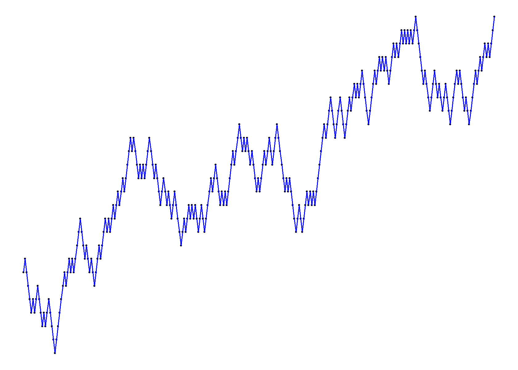
Let us start with a basic simulation of a random walk by considering a heavily drunk man who has completely lost his mind, yet determined to take every step regardless, and wanders around in an erratic fashion. For this example, we assume the man can only move one unit either to his right or left of his current position. A trace of the paths taken by this man in a 300-walk, for instance, can be simulated in R with the vectorized cumsum() function. (Note: we assume $P(X_1 = -1) = P(X_1 = 1) = 1/2$). The visualization is shown below.

library("tidyverse")
set.seed(2021-09-22)
n <- 300 # 300 random walks
data.frame(x = 1:n, y = cumsum(sample(c(1,-1), n, replace=TRUE))) %>%
  ggplot(aes(x=x, y=y)) + 
  geom_point(size = 0.5) + geom_path(color = "blue") +
  theme_void()

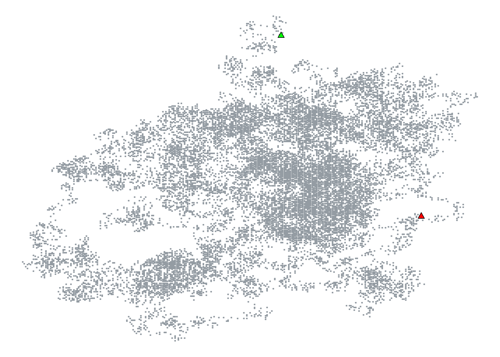
The random walk above only considered the direction of the movement (right or left), without special focus to varying distances space. In the following illustration, we shall be simulating a random walk that takes into consideration the displacement from the drunk man’s current position. We consider a displacement space of ${0, 1, 2, 3, 4}$ in both directions, thus, $\mbox{displacement} = \{-4, -3, \ldots, 3, 4\}$. We demonstrate one instance of the walk, with $size = 20000$ random walks. The green triangle marks the starting point whiles the red triangle marks the final destination (step 20000). We shall also provide a link to a shinyApp where you may play around with different simulation sizes, and get to see interesting plots each time the simulation type is varied.

x_values = 0
y_values = 0

distance_space <- c(0, 1, 2, 3, 4)
displacement <- c(-1, 1)

set.seed(2021-09-22)
num = 1 # looping point
steps = 20000 # random walks to generate

# data generation
while (num < steps) {
  walked <- replicate(2, sample(displacement, size = 1, replace = TRUE) * 
                                        sample(distance_space, size = 1, replace = TRUE))
  # disregard (0,0)
  if(walked[1] == 0 && walked[2] == 0) 
    next
  x_values[num+1] = walked[1] + x_values[num]
  y_values[num+1] = walked[2] + y_values[num]
  num = num + 1
}

dat <- data.frame(x_values, y_values)
            
# plot random walks
dat %>%
  ggplot(aes(x = x_values, y_values)) + 
                #geom_path(color = input$col) +
                geom_point(size = 0.35, color = "#949CA3") +
                theme_void() +
                theme(axis.title=element_blank(),
                      axis.text=element_blank(),
                      axis.ticks=element_blank()) + #,
                geom_point(data = dat[1,], aes(x = x_values, y = y_values),
                           fill = "green", shape = 24, size = 2) + 
                geom_point(data = dat[steps,], aes(x = x_values, y = y_values), 
                           fill = "red", shape = 24, size = 2)

For this random walk of size $20000$ is fairly large enough (subjectively). What does the figure look like?. Well, it looks like a cloud-like sky — wispy sort of. Okay, what happens if we increase the simulation size to, say, $50000$ or more, what would the shape look like? Again, from the above figure, looking at the starting point (green button) and final point (red button), we may guess stochasticity is well represented in the figure. In other words, knowing the current position of the drunk man, we do not know in advance where exactly his next position will be. Thus, nondeterministic-ally, we are unable to predict exactly the final shape of the figure. However, we are well sure to say that, as the simulation size increases, we tend to lose the visual appeal of the plot (as overplotting setting in). Not convinced? Follow the simple instructions below to see this (shinyApp):

Visit the the link: ssalpawuni shinyApp
Use the slider button to change the number of simulations (between 10-50K)
Use the tick box to see where the simulation started and where it ended
Use the color picker window to choose your preferred color
Wait for the simulation result (about 20 seconds!)

Any suggestions? Did you find this post helpful? You may consider sharing it😊😊😊