In Statistics, estimating uncertainty of an unknown quantity is a core problem. Broadly speaking, dealing with this can take one of two paths — Frequentist estimation or Bayesian estimation. It is worth noting, however, that these two approaches fundamentally have different inference schemes about how they express degree of belief, and needless to say, there is a raging 2-century-old debate over what probability means. In this post, I intend to briefly focus on Bayesian statistics, with demonstrations in R. Basic knowledge of Statistics is assumed. Further to that, I assume you have, at least, a basic working familiarity with analysis in R Software.

Let us assume I show you a flip coin and exclaimed; ‘Look! This coin in my hand is unbias’. But you are not the type of people to accept mere assertions without overwhelming evidence. So to accept my claim, you demand that we toss the coin, say, $1000$ times, and count the number of times ‘heads’ showed up relative to the number of ‘tails’ produced. Now, if my claim were right, we expect a close proportion of heads and tails, say, for example, $510$-heads to $490$-tails. However, if in a $1000$-toss, it turned out that, $999$ cases landed on a ‘head’, and only one landed on a ‘tail’, then you would have had overwhelming evidence against my claim, outrightly rejecting the claim of ‘unbiasedness’. Even so, if the probability of head were 0.75 or 0.15 or some value other than 0.50, that would still be a piece of evidence against my claim. To express this statistically, we may represent this experiment as one that follows a binomial distribution as;

$$X_n\sim \text{Binom}(\theta ,n);$$ where $\theta$ is the probability of landing a head (parameter) from trial to trial, and $n$ is the number of flips in the experiment.

Referring to the representation above, if we consider $\theta$ in the classical setting where the parameter has a fixed (either known or unknown), then it absolutely makes no sense to ask a question like $P({\theta }_1<\theta <{\theta }_2|X_n,n)=?$. This is so because, the Frequentist approach treats the parameter as a fixed quantity with no room for variation, and can only be estimated through repeated sampling, under identical conditions. Thus, Frequentist statistics depends on the long-run frequency of the trials. In contrast, for Bayesian setting, the fact that a parameter is fixed is completely rejected in that, it is treated as a random variable having some probability distribution. In fact, we start estimation with an initial belief (called the prior) before we even see/observe the data. After looking at the data, our belief of the parameter (estimation) is updated (posterior). It is because of the subjective nature of the ‘initial belief’ that makes many frequentist enthusiasts criticize the Bayesian method. However, Bayesian statisticians have refuted this criticism by positing that, in decision-making where uncertainty is present, it’s better to explore all scenarios in a rigorous and coherent manner. I should point out immediately that, these two approaches are not, in reality, contradictory but only presents us an opportunity to address the problem from two different angles.

Template for Bayesian inference

In this section, I will briefly illustrate the so-called ‘prototype’ of Bayesian statistical inference. Let $\theta$ represent a parameter of interest that is considered unknown. Furthermore, let $y$ be the observed data. Therefore, a Bayesian inference can be formulated as;

$$\begin{array}{rl}P(\theta |y)& =\frac{P(\theta )P(y|\theta )}{P(y)}\\ P(\theta |\text{data})& =\frac{P(\theta )P(\text{data}|\theta )}{\int P(\theta )P(\text{data}|\theta )d\theta }\\ \text{posterior}& =\frac{\text{prior}\times \text{likelihood}}{\text{averag-likelihood}}\end{array}$$

where;

• $p(\theta )$ is the prior. The plausible values of $\theta$ before we see the data
• $p(y|\theta )=L(\theta ;y)$ is the likelihood. The sampling distribution relative to the unknown parameters.
• $p(\theta |y)$ is the posterior. After seeing the data, what is our updated belief?
• $p(y)$ is the normalizer. A constant that is of less importance to the modeling process

Example

In a certain population, it is believed that $1.5\mathrm{\%}$ of the population have disease X. Assuming health providers in that community decide to embark on a free screening exercise for the said disease. And it is known that, for a person who has the disease, the test has an accuracy of $97\mathrm{\%}$ for a positive test result. Also, for a person who does not have the disease, the test has an accuracy of $95\mathrm{\%}$ for a negative test result. Assuming you presented yourself for testing and your test result came out positive for the disease. what is the probability that you actually have the disease?

This is clearly a Bayesian problem. Define $D$ as an event that a subject has the disease, $T^{+}$ be event that a subject’s test result returns positive, and the event that a subject’s test result $T^{-}$ returns negative. Thus far, we proceed with the following pieces of information;

$$\begin{array}{rl}P(D)& =0.015\text{(prevalence)}\\ P(T^{+}|D)& =0.97\text{(sensitivity)}\\ P(T^{-}|D^{\prime })& =0.95\text{(specificity)}\end{array}$$

We’re interested in $P(D|T^{+})$, the probability you have the disease given you tested positive to the disease. Using the Bayesian formulation, we proceed as follows:

$$\begin{array}{rl}P(D|T^{+})& =\frac{P(D)P(T^{+}|D)}{P(D)P(T^{+}|D)+P(D^{\prime })P(T^{+}|D^{\prime })}\\ & =\frac{0.015\times 0.97}{0.015\times 0.97+(1-0.015)\times (1-0.95)}\\ & =\frac{0.01455}{0.905975}\\ & =0.0161\end{array}$$

So what is this value? It represents our updated belief of the proportion of people in the population who are having the disease, thus, $1.61\mathrm{\%}$. In other words, were we not to use the Bayesian method, we would not have been able to have an updated version of the prevalence of the disease in the population.

From this simple demonstration, let’s move to a more interesting scenario; a case where we allow the prior to take more plausible values (rather than a point estimate), observed data, and the likelihood. I shall demonstrate this in R using ‘brute force’. One way to do that is to consider $\theta$ where we have no prior information about it. So we want to consider all possible values of it by letting it follow, for example, a uniform distribution (more generally, beta distribution). In the plot below, I have varied the beta distribution for flexibility, for six different shape values. Each graph conveys a piece of different prior information. (See: Fong Chun Chan)

xfun::pkg_attach(c("tidyverse", "glue", "cowplot"))

beta_params <-
  tribble(
    ~ shape1, ~ shape2,
      0.5,      0.5,
      1.0,      1.0,
      5.0,      1.5,
      5.0,      5.0,
      5.0,      20.0,
      50.0,     150.0
    )

# Create plot of beta distribution with varying shapes
plot_beta <- function(dat) {
  shap1 <- dat[["shape1"]]
  shap2 <- dat[["shape2"]]

  data.frame(x = c(0, 1)) %>%
    ggplot(aes(x)) +
    stat_function(
      fun = dbeta,
      n = 101,
      args = list(shape1 = shap1, shape2 = shap2)
    ) +
    ylab("Density") +
    xlab("Probability") +
    ggtitle(glue("Beta({shap1}, {shap2})")) + theme_grey()
}

beta_plots <-
  split(beta_params, seq_len(nrow(beta_params))) %>%
  lapply(plot_beta)

plot_grid(
  plotlist = beta_plots,
  ncol = 3, nrow = 2,
  labels = c("I", "II", "III", "IV", "V", "VI"),
  align = "none",
  label_size = 11
)

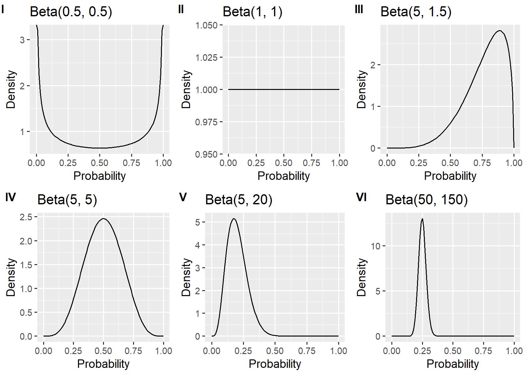
In practice, you could set the prior to any probability distribution of your choice, but some known probability distributions make the maths easier to handle. For instance, if we cite the earlier example (about screening a disease X), it is reasonable to think that the number of people who tested positive for the disease follows a binomial distribution with an unknown parameter, $\theta$. Further to that, if we set the prior to follow a beta distribution, it can be shown that $\theta |y$ also follows a beta distribution. This is what is Bayesian statisticians termed as “conjugacy”, meaning that the posterior distribution has the same parametric form as that of the prior distribution (i.e. the beta distribution is a conjugate prior to the binomial distribution). For more details on this, see towards data science.

Now, consider a hypothetical situation where you decide to check your inbox (email) for incoming messages. Let’s say you do the checking only between $10.00$am and $12.00$pm for the next 20 days. It turned out that, out of the $20$ days, you actually received email(s) on $5$ days. But before this observation, it is fair to assume that you had no prior knowledge regarding the probability of receiving at least one email between $10.00$am and $12.00$pm. So we want to estimate this probability (i.e. our $\hat{\theta }$). You could start this by assuming that emails hit your inbox in a uniform fashion ($X\sim Beta(1,1)$) throughout the period. Below, I shall allow the prior to assume various forms, keeping in mind that the number of emails in the $20$-day trial follows a binomial distribution. The code below accomplishes this task. The goal is to see the form of the prior, likelihood, posterior forms.

xfun::pkg_attach(c("tidyverse", "reshape2", "glue", "cowplot"))

data = 5
beta_params <-
  tribble(
    ~ shape1, ~ shape2,
    0.5,      0.5,
    1,        1,
    5,        1,
    5,        5,
    15,       5,
    50,     160
  )
plot_beta <- function(dat) {
  # extract shape1 and shape2 values
  cur_shape_1 <- dat[["shape1"]]
  cur_shape_2 <- dat[["shape2"]]

  param_space <- seq(0, 1, by = 0.001) # parameter space
  likelihood <- dbinom(data, size = 20, prob = param_space) # Likelihood
  prior <- dbeta(param_space, shape1 = cur_shape_1, shape2 = cur_shape_2) # Prior
  weighted_likelihood <- likelihood * prior # numerator
  normalizer <- sum(weighted_likelihood) # denominator
  posterior <- weighted_likelihood/normalizer # posterior distribution

  my_dat <-
    melt(data =
           tibble(
             Theta = param_space,
             Likelihood = likelihood * 5,
             Prior = prior,
             Posterior = posterior*length(param_space)
           ),
         id.vars = "Theta",
         variable.name = "Key"
    )

  ggplot(my_dat, aes(x = Theta, y = value, color = Key)) +
    geom_path() +
    ylab("Probability density") +
    xlab("Parameter space (theta)") +
    ggtitle(glue("Beta({cur_shape_1}, {cur_shape_2})"))
}

beta_plots <-
  split(beta_params, seq_len(nrow(beta_params))) %>%
  lapply(plot_beta)

# Combined plotting
plot_grid(
  plotlist = beta_plots,
  ncol = 2, nrow = 3,
  labels = c("I", "II", "III", "IV", "V", "VI"),
  align = "none",
  label_size = 11
)

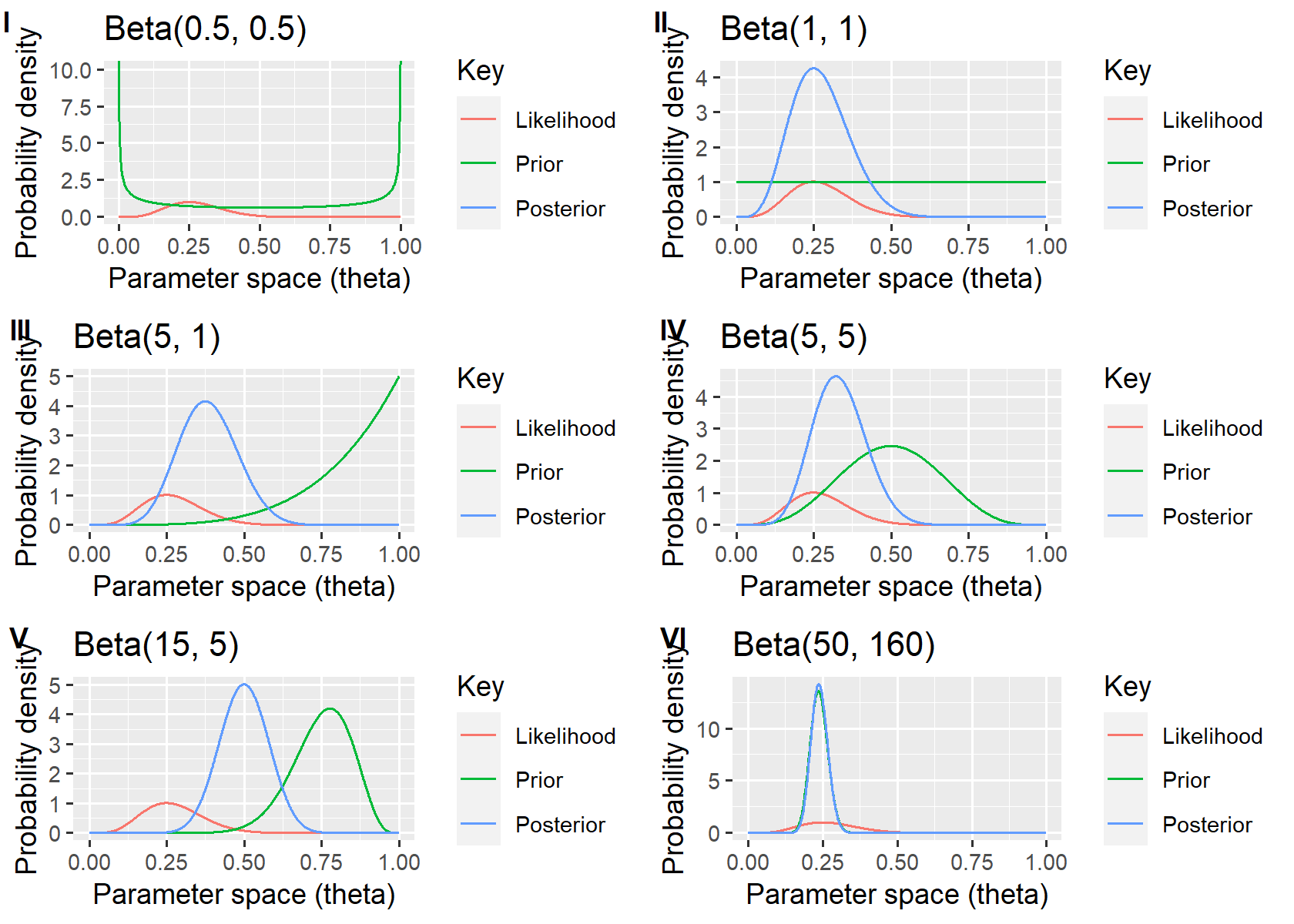
From the figure, taking for example $\text{Beta}$(1, 1), clearly, we see that the prior has the same parametric form as the likelihood surface. What information does this convey to us? Actually, it gives an indication that, the prior has been overwhelmed by the amount of information contained in the data we observe. In other words, it represents the global uncertainty that the probability of receiving an email between the times $10.00$am and $12.00$pm could be any value in the interval. What about $\text{Beta}$(0.5, 0.5)? Well, it represents a belief that an email(s) is(are) received or not received between the given interval.

Concluding remarks

In this post, I have briefly touched on Bayesian Statistics – where we start the estimation process with an initial ‘belief’, and as the modeling processes continue, we get to update the so-called belief. Thus, before we look at the data, what possible is the value of the parameter, $\theta$? After we see the data, how is our belief of it ‘updated’? As you might have realized, I have dealt only with non-informative prior as against informative priors which generally incorporate external information into the modeling process. For instance, in our ‘email experiment’, we dealt with one trial, relying on ‘non-informative prior’. To go deeper, we could have decided to collect more data, by way of repeating the trials several times, and investigating the behavior of the estimation for a prior, for instance, $\text{Beta}$(150, 5). Finally, this post did not touch on ‘credible intervals’, finding Bayesian point estimates, and many more. A comprehensive discussion of these is well beyond this post.

Did you find this post helpful? Consider sharing it😊😊😊